Dealing with a massive Excel sheet? Freezing panes or splitting the screen can make navigation easier and help you stay oriented.
Freeze panes: keep rows or columns visible
The Freeze Pane feature allows you to keep certain rows or columns visible while you scroll through your sheet. It‘s ideal for:
- Keep column headings visible
- Track data without losing context
- Work on large sheets without confusion
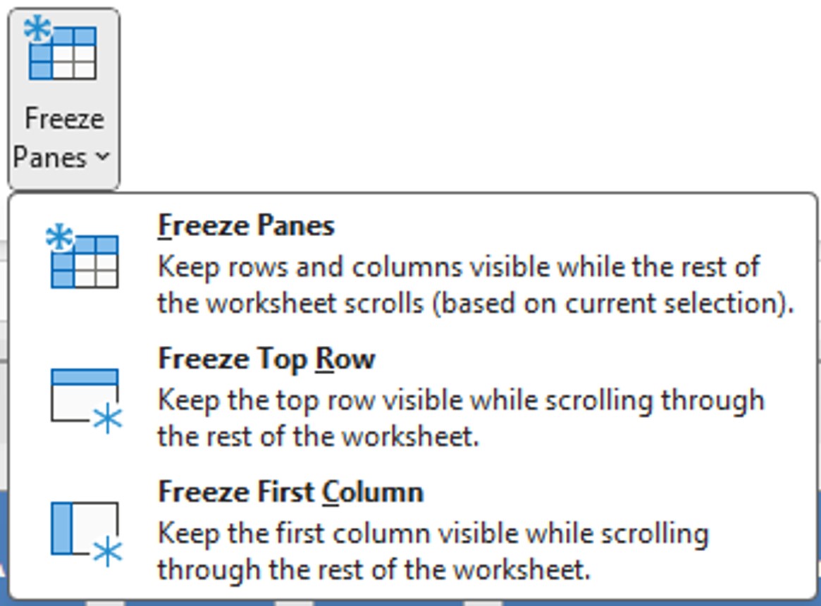
The Freeze Panes menu offers 3 options:
- Freeze Panes: Keeps the rows above and columns to the left of the selected cell visible.
- Freeze Top Row: Keeps the first line visible.
- Freeze First Column: Keeps the first column visible.
Freeze Top Row
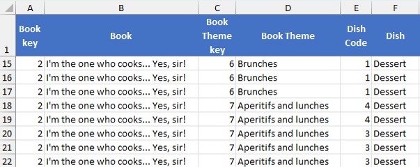
When you choose this option, the 1st row of your table is frozen. So when you scroll through your sheet, it always stays in view.
- Go to the View tab.
- Click Freeze Panes.
- Select Freeze Top Row.
Useful for keeping headers visible while scrolling vertically.
Freeze First Column
- On the View tab, click Freeze Panes.
- Choose Freeze First Column.
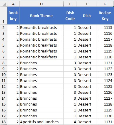
Perfect for tracking names or IDs when scrolling horizontally.
In our example, we can see that column D follows column A on display.
Freeze multiple rows and/or columns
The Freeze Pane option (the default) is special. This is because the rows and columns will be frozen depending on where your cursor is located.
When a cell is selected, all columns to the left of the selected cell are frozen, and all rows at the top of that cell are frozen.
- Select the cell just below the rows and to the right of the columns you want to freeze.
- Click View > Freeze Panes > Freeze Panes
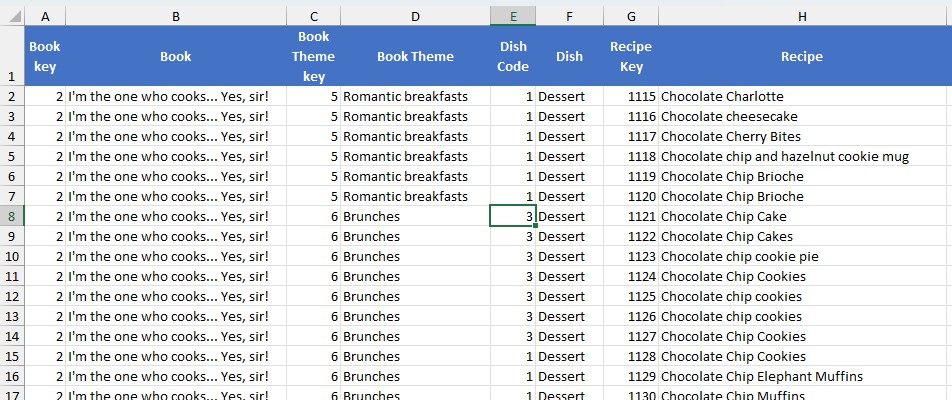
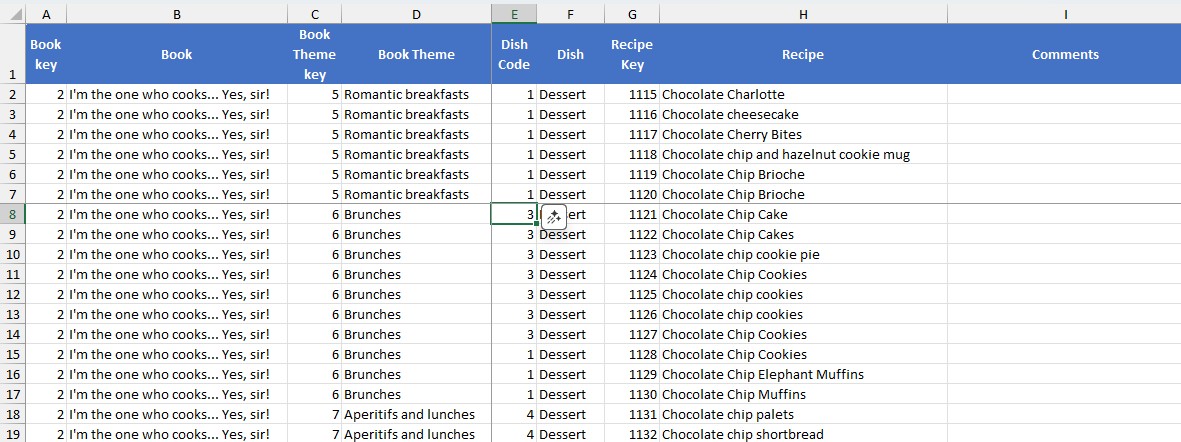
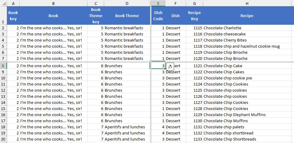
In our example, cell E8 is selected. Columns A to D and rows 1 to 7 are thus fixed.
When you scroll through the table, these rows and columns are still visible.
Tip: Sometimes you get a file that seems impossible to navigate. Check that the panes are not frozen.
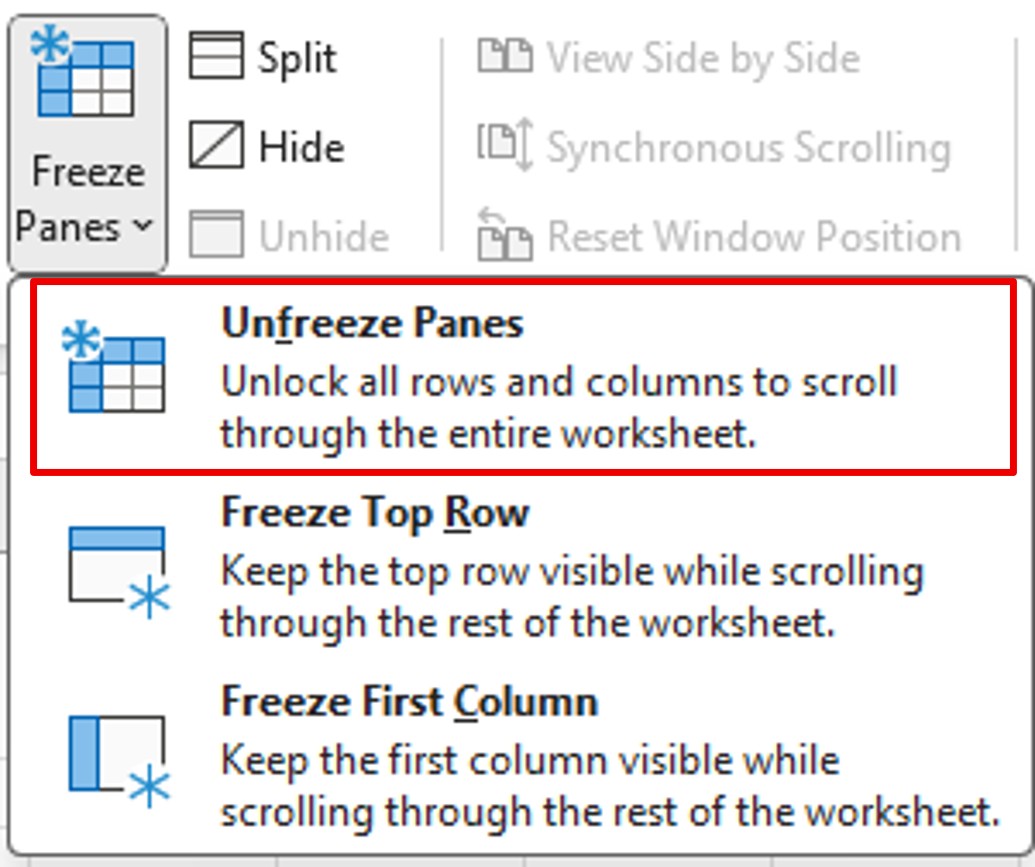
Unfreeze Panes
Split Screen: For a Parallel View
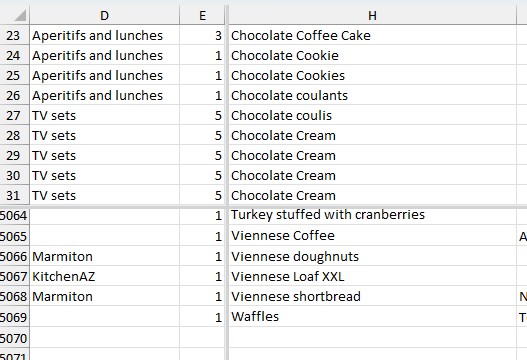
The Split function allows you to divide the Excel window into several viewing areas. Each area can be scrolled independently.
A scenario in the article: Excel : Copier et coller une formule sur une ou plusieurs colonnes, même en présence de cellules vides
To delete the fraction:
Click Split again to turn off the split view.
Summary of functions
| Function | Main Utility | Quick Access |
|---|---|---|
| Freeze top row | Keep titles visible by scrolling | View > Freeze panes |
| Freeze the first column | Track IDs | View > Freeze panes |
| Freeze Multiple Panes | Large Sheet Navigation | Selection + Freeze Panes |
| Split Screen | Parallel View of Multiple Zones | View > Split |


