

Want to retrieve data from a source table to a target table? Is the lookup value not on the left?
Sometimes, the Vlookup and Hlookup functions are not enough. Xlookup is more flexible, allowing more advanced searches… just as easily.
Why use XLOOKUP
XLOOKUP makes it easy to retrieve data from a source table into a target table. It offers a more flexible search than VLOOKUP:
- No matter where the lookup value is located – it doesn’t need to be on the left.
- It can return multiple contiguous columns at once.
- It can display an alternative value if the lookup fails.
- And many other advanced options.
Definition
The XLOOKUP function, accessible on Microsoft 365 and Excel 2021+, looks like this:
=XLOOKUP(lookup_value, lookup_array, return_array, [if_not_found], [match_mode], [search_mode])
Lookup value
A value (in the target array) that you want to match.
Lookup array
Column (in the source table) containing the data you are looking for.
Note: The lookup array can be anywhere in your workshette – it doesn’t need to be to the left of the return array.
Return array
Column containing the data to be repatriated. It is possible to retrieve data from several contiguous columns.
If not found
Optional value. If the value you are looking for is not in the search table, you can display a value, a word surrounded by ““ (e.g. “Not OK“) or even a function: no need to use a function such as IFERROR!
Match mode
Optional value. Choosing the desired value match:
- Exact Match
- Exact Match or Next Lower Item
- Exact Match or Next Higher Item
- Wildcard Matching
Search mode
An optional value. This argument allows you to choose an inverse or other search mode:
- Search from the first to the last
- Searching from last to first
- Binary search (sort ascending)
- Binary search (sort descending)
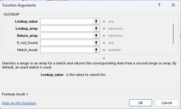
To display the Search Mode field, scroll down using the scrollbar.
Practical exemple
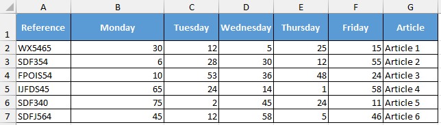
From the following table (source table), we will retrieve data into another table.
Finding value
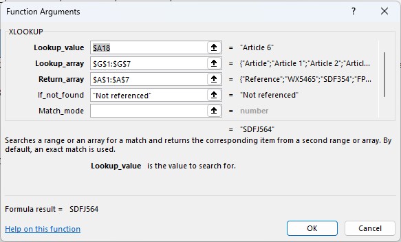
In the table below, we would like to retrieve the item reference.
For the 1st row (line 11), with the XLOOKUP function, we search for “Item 6“ (A11, from the target table); in the column where it is in the reference table (G1:G7, from the source table) to retrieve the reference (A1:A7, from the source table). If the value we are looking for is not found, then the result shows “Not referenced“.
This gives us the following formula:
=XLOOKUP($A1/;$G$1:$G$7;$A$1:$A$7;”Not referenced”)

Search for multiple values
To do this, for the 1st row (row 11), we search for “Article 6“ (A11, from the target table); in the column where it is in the reference table (G1:G7, from the source table) to retrieve the data for the days of the week (B1:F7, from the source table). If the value we are looking for is not found, then the result returns an empty string (““).
This gives us the following formula:
=XLOOKUP($A11;$G$1:$G$7;$B$1:$F$7;””)

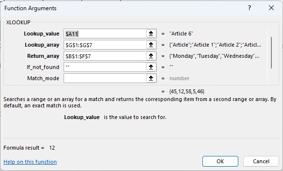
Note: the formula is entered in the first column and the results propagate in the other columns. These cells must be empty, otherwise the spill will be blocked.